![]()
Galveston Testbed (previous version)#
IN-CORE Flowchart - Galveston#
This notebook uses the Galveston testbed to demonstrate the following components of the IN-CORE flowchart.

Background#
The Galveston Testbed is an ongoing effort of the Center to test model chaining an integration across coupled systems. The current Galveston Testbed and Jupyter notebooks released with IN-CORE focus on Galveston Island as a barrier island exposed to hurricane hazards. Our ongoing work extends this analysis to Galveston County, further exploring the interplay between economic activity and recovery efforts between the mainland and the island. As shown in the following figure, Galveston County is located in the southeastern part of Texas, along the Gulf Coast adjacent to Galveston Bay.
Galveston Island is located in southern Galveston County with a total length of 43.5 km and a width of 4.8 km. The Island is surrounded by West Bay from the west, the Gulf of Mexico from the south and east, and Galveston Bay in the North. The Galveston Island is connected to the rest of Galveston County by interstate highway I-45. Based on the 2015 county parcel data the total number of buildings within Galveston County was 172,534 buildings with 29,541 buildings located on Galveston Island. In 2010, the total population living on Galveston Island was 48,726 people with a racial/ethnic composition of 46% non-Hispanic White, 18% non-Hispanic Black, and 31% Hispanic. Galveston, Texas has a long history with hurricanes including the Great Galveston Hurricane in 1900 which is considered the deadliest natural disaster in U.S. history. More recently, the island was affected by Hurricane Ike (2008) and Hurricane Harvey (2017), each posing unique challenges in terms of coastal multi-hazards and recovery challenges, and with billions of dollars in economic impacts.

General info#
Some of the main objectives of the Galveston Testbed include:
Investigate the multi-hazard surge, wave, inundation, and wind hazards in coastal settings.
Consider interdependent infrastructure systems including buildings, transportation, and power.
Leverage historical social-science data, informing population dislocation and recovery modeling.
Evaluate hybrid metrics of community resilience, such as those that require coupled modeling between social and physical systems.
More information about the testbed and the field study can be found in this publication:
Fereshtehnejad, E., Gidaris, I., Rosenheim, N., Tomiczek, T., Padgett, J. E., Cox, D. T., … & Gillis Peacock, W. (2021). Probabilistic risk assessment of coupled natural-physical-social systems: cascading impact of hurricane-induced damages to civil infrastructure in Galveston, Texas. Natural Hazards Review, 22(3), 04021013.
The current notebook is a WORK-IN-PROGRESS that consists of the following modules:
Community Description with Housing Unit Allocation
Hazard Model: Flood Surge, Wave, and Inundation Modeling with Building Damage
Functionality Models: Phycial Infrastructure and Population Dislocation
Recovery Models with Household-Level Housing Recovery Analysis
Policy Lever Analysis
The models used in this testbed come from:
Nofal, O. M., Van De Lindt, J. W., Do, T. Q., Yan, G., Hamideh, S., Cox, D. T., & Dietrich, J. C. (2021). Methodology for Regional Multihazard Hurricane Damage and Risk Assessment. Journal of Structural Engineering, 147(11), 04021185.
Darestani, Y. M., Webb, B., Padgett, J. E., Pennison, G., & Fereshtehnejad, E. (2021). Fragility Analysis of Coastal Roadways and Performance Assessment of Coastal Transportation Systems Subjected to Storm Hazards. Journal of Performance of Constructed Facilities, 35(6), 04021088.
Darestani, Y., Padgett, J., & Shafieezadeh, A. (2022). Parametrized Wind–Surge–Wave Fragility Functions for Wood Utility Poles. Journal of Structural Engineering, 148(6), 04022057.
Rosenheim, N., Guidotti, R., Gardoni, P., & Peacock, W. G. (2019). Integration of detailed household and housing unit characteristic data with critical infrastructure for post-hazard resilience modeling. Sustainable and Resilient Infrastructure, 6(6), 385-401.
Sutley, E. J., & Hamideh, S. (2020). Postdisaster housing stages: a markov chain approach to model sequences and duration based on social vulnerability. Risk Analysis, 40(12), 2675-2695.
Prerequisites: The following packages are necessary to run this notebook. To ensure dependencies are correct, install all modules through conda.
Module |
Version |
Notes |
|---|---|---|
pyIncore |
=>1.7.0 |
see: https://incore.ncsa.illinois.edu/doc/incore/install_pyincore.html |
pyIncore_viz |
=>1.5.0 |
see: https://incore.ncsa.illinois.edu/doc/pyincore_viz/index.html |
Start#

The following codes are preparing the analysis by checking versions and connecting to IN-CORE web service. Also, all of the necessary pyIncore analyses are being imported. In this analysis, the following pyIncore analyses are utilized:
Building damage: Computes building damage based on a particular hazard (hurricane in this testbed).
Building functionality: Calculates building functionality probabilities.
Housing unit allocation: Sets up a detailed critical infrastructure inventory with housing unit level characteristics.
Population dislocation: Computes population dislocation based on a particular hazard (hurricane in this testbed).
Household-level housing sequential recovery: Computes the series of household recovery states given a population dislocation dataset.
Policy Lever Demonstration: Modify Building Inventory to reduce building damage.
import warnings
warnings.filterwarnings("ignore")
import pandas as pd
import geopandas as gpd
import numpy as np
import sys
import os
import matplotlib.pyplot as plt
import contextily as ctx
import copy
import math
from scipy.stats import norm
from pathlib import Path

from pyincore import IncoreClient, Dataset, DataService, HazardService, FragilityService, MappingSet, FragilityCurveSet
from pyincore_viz.geoutil import GeoUtil as geoviz
from pyincore_viz.plotutil import PlotUtil as plotviz

# importing pyIncone analyses:
from pyincore.analyses.buildingdamage import BuildingDamage
from pyincore.analyses.bridgedamage import BridgeDamage
from pyincore.analyses.buildingfunctionality import BuildingFunctionality
from pyincore.analyses.combinedwindwavesurgebuildingdamage import CombinedWindWaveSurgeBuildingDamage
from pyincore.analyses.epfdamage import EpfDamage
from pyincore.analyses.housingunitallocation import HousingUnitAllocation
from pyincore.analyses.populationdislocation import PopulationDislocation, PopulationDislocationUtil
from pyincore.analyses.housingrecoverysequential import HousingRecoverySequential
from pyincore.analyses.socialvulnerability import SocialVulnerability
---------------------------------------------------------------------------
ModuleNotFoundError                       Traceback (most recent call last)
Cell In[1], line 3
      1 import warnings
      2 warnings.filterwarnings("ignore")
----> 3 import pandas as pd
      4 import geopandas as gpd
      5 import numpy as np

ModuleNotFoundError: No module named 'pandas'
# Functions for visualizing the population data results as tables
from pyincore_viz.analysis.popresultstable import PopResultsTable as poptable
# Check package versions - good practice for replication
print("Python Version ", sys.version)
print("pandas version: ", pd.__version__)
print("numpy version: ", np.__version__)
Python Version  3.9.15 | packaged by conda-forge | (main, Nov 22 2022, 08:41:22) [MSC v.1929 64 bit (AMD64)]
pandas version:  1.5.2
numpy version:  1.24.1
# Check working directory - good practice for relative path access
os.getcwd()
'C:\\Users\\ka50\\Box\\Rice\\Software_Projects\\Pycharm\\IN-CORE_Galveston\\jupyter_book\\notebooks'
client = IncoreClient()
# IN-CORE caches files on the local machine, it might be necessary to clear the memory
# client.clear_cache()
data_service = DataService(client) # create data_service object for loading files
hazard_service = HazardService(client)
fragility_services = FragilityService(client)
Connection successful to IN-CORE services. pyIncore version detected: 1.8.0
1) Initial community description#

Step 1 in IN-CORE is to establish initial community description at time 0 and with policy levers and decision combinations (PD) set to K (baseline case). The community description includes three parts including 1a) Built Environment, 1b) Social Systems, and 1c) Economic Systems.
1a) Built Environment#
The Galveston testbed consists of five infrastructure systems as buildings, transportation network, electric power transmission and distribution network, water/wastewater network, and critical facilities. Each infrastructure system may be composed of different infrastructure components. For example, the transportation network consists of bridges and roadways. The infrastructure systems and components are shown below along with their IN-CORE GUID.
No. |
Infrastructure System |
Infrastructure Component |
GUID |
More details |
|---|---|---|---|---|
1 |
Buildings |
- |
63053ddaf5438e1f8c517fed |
Ref. |
2 |
Transportation network |
Bridges |
60620320be94522d1cb9f7f0 |
Ref. |
- |
Transportation network |
Roadways |
5f15d04f33b2700c11fc9c4e |
Ref. |
3 |
Electric power network |
Connectivity |
Outside of IN-CORE |
Ref. |
- |
Electric power network |
Poles and Towers |
Outside of IN-CORE |
Ref. |
- |
Electric power network |
Substation |
Outside of IN-CORE |
Ref. |
- |
Electric power network |
Transmission |
Outside of IN-CORE |
Ref. |
- |
Electric power network |
Underground |
Outside of IN-CORE |
Ref. |
4 |
Water/wastewater network |
Water mains |
Outside of IN-CORE |
Ref. |
- |
Water/wastewater network |
Water plants |
Outside of IN-CORE |
Ref. |
- |
Water/wastewater network |
Wastewater mains |
Outside of IN-CORE |
Ref. |
5 |
Critical facilities |
Hospitals |
Outside of IN-CORE |
Ref. |
- |
Critical facilities |
Urgent care |
Outside of IN-CORE |
Ref. |
- |
Critical facilities |
Emergency medical facilities |
Outside of IN-CORE |
Ref. |
- |
Critical facilities |
Fire stations |
Outside of IN-CORE |
Ref. |
6 |
Fiber Optic Network |
- |
Outside of IN-CORE |
Ref. |
Note: The built environment in the Galveston testbed are in the Galveston Island. However, as the goal is to capture flow of people during recovery stages, buildings and transportation networks in the Galveston mainland are considered as well.
Buildings#
The building inventory for Galveston consists of 172,534 individual buildings. This inventory is also mappable to housing unit info of 132,553 individual households explained later in this notebook. It should be noted that the reason that the building and household data are different in terms of numbers is that each individual building can be composed of a few households or no households in the case of commercial or industrial buildings. The building inventory consists of major parameters that are used to estimate the fragility of buildings explained shortly later in this notebook.
bldg_dataset_id = "63053ddaf5438e1f8c517fed" # Prod              # defining building dataset (GIS point layer)

bldg_dataset = Dataset.from_data_service(bldg_dataset_id, data_service)
# geoviz.plot_map(bldg_dataset, column='arch_flood',category='True')
print('Galveston testbed building inventory as a function of age group')

bldg_df = bldg_dataset.get_dataframe_from_shapefile()
#bldg_df.set_index('guid', inplace=True)
print('Number of buildings: {}' .format(len(bldg_df)))
Dataset already exists locally. Reading from local cached zip.
Unzipped folder found in the local cache. Reading from it...
Galveston testbed building inventory as a function of age group
Number of buildings: 172534
1a + 1b) Interdependent Community Description#
Explore building inventory and social systems. Specifically look at how the building inventory connects with the housing unit inventory using the housing unit allocation. The housing unit allocation method will provide detail demographic characteristics for the community allocated to each structure.
To run the HUA Algorithm, three input datasets are required:
Housing Unit Inventory - Based on 2010 US Census Block Level Data
Address Point Inventory - A list of all possible residential/business address points in a community. Address points are the link between buildings and housing units.
Building Inventory - A list of all buildings within a community.
Set Up and Run Housing Unit Allocation#
The building and housing unit inventories have already by loaded. The address point inventory is needed to link the population with the structures.
# Create housing allocation
hua = HousingUnitAllocation(client)

address_point_inv_id = "6320da3661fe1122867c2fa2"

# Load input dataset
hua.load_remote_input_dataset("housing_unit_inventory", housing_unit_inv_id)
hua.load_remote_input_dataset("address_point_inventory", address_point_inv_id)
hua.load_remote_input_dataset("buildings", bldg_dataset_id)

# Specify the result name
result_name = "Galveston_HUA"

seed = 1238
iterations = 1

# Set analysis parameters
hua.set_parameter("result_name", result_name)
hua.set_parameter("seed", seed)
hua.set_parameter("iterations", iterations)
---------------------------------------------------------------------------
HTTPError                                 Traceback (most recent call last)
Cell In[19], line 7
      4 address_point_inv_id = "6320da3661fe1122867c2fa2"
      6 # Load input dataset
----> 7 hua.load_remote_input_dataset("housing_unit_inventory", housing_unit_inv_id)
      8 hua.load_remote_input_dataset("address_point_inventory", address_point_inv_id)
      9 hua.load_remote_input_dataset("buildings", bldg_dataset_id)

File ~\Anaconda3\envs\IN-CORE_GAlveston\lib\site-packages\pyincore\baseanalysis.py:72, in BaseAnalysis.load_remote_input_dataset(self, analysis_param_id, remote_id)
     64 def load_remote_input_dataset(self, analysis_param_id, remote_id):
     65     """Convenience function for loading a remote dataset by id.
     66
     67     Args:
   (...)
     70
     71     """
---> 72     dataset = Dataset.from_data_service(remote_id, self.data_service)
     74     # TODO: Need to handle failing to set input dataset.
     75     self.set_input_dataset(analysis_param_id, dataset)

File ~\Anaconda3\envs\IN-CORE_GAlveston\lib\site-packages\pyincore\dataset.py:57, in Dataset.from_data_service(cls, id, data_service)
     45 @classmethod
     46 def from_data_service(cls, id: str, data_service: DataService):
     47     """Get Dataset from Data service, get metadata as well.
     48
     49     Args:
   (...)
     55
     56     """
---> 57     metadata = data_service.get_dataset_metadata(id)
     58     instance = cls(metadata)
     59     instance.cache_files(data_service)

File ~\Anaconda3\envs\IN-CORE_GAlveston\lib\site-packages\pyincore\dataservice.py:47, in DataService.get_dataset_metadata(self, dataset_id)
     45 # construct url with service, dataset api, and id
     46 url = urljoin(self.base_url, dataset_id)
---> 47 r = self.client.get(url)
     48 return r.json()

File ~\Anaconda3\envs\IN-CORE_GAlveston\lib\site-packages\pyincore\client.py:314, in IncoreClient.get(self, url, params, timeout, **kwargs)
    311     self.login()
    312     r = self.session.get(url, params=params, timeout=timeout, **kwargs)
--> 314 return self.return_http_response(r)

File ~\Anaconda3\envs\IN-CORE_GAlveston\lib\site-packages\pyincore\client.py:166, in Client.return_http_response(http_response)
    163 @staticmethod
    164 def return_http_response(http_response):
    165     try:
--> 166         http_response.raise_for_status()
    167         return http_response
    168     except requests.exceptions.HTTPError:

File ~\Anaconda3\envs\IN-CORE_GAlveston\lib\site-packages\requests\models.py:1021, in Response.raise_for_status(self)
   1016     http_error_msg = (
   1017         f"{self.status_code} Server Error: {reason} for url: {self.url}"
   1018     )
   1020 if http_error_msg:
-> 1021     raise HTTPError(http_error_msg, response=self)

HTTPError: 403 Client Error: Forbidden for url: https://incore.ncsa.illinois.edu/data/api/datasets/626322a7e74a5c2dfb3a72b0
# Run Housing unit allocation analysis - temporarily disabled - read from dataset instead
# hua.run_analysis()
Explore results from Housing Unit Allocation#
# Retrieve result dataset
# hua_result = hua.get_output_dataset("result")
# NOTE to USER - pyincore 1.7.0 has internal error and this notebook includes a workaround for the HUA analysis
hua_result_id = "6328a9b873b4ed0eefbacad6"

hua_result = Dataset.from_data_service(hua_result_id, data_service)

# Convert dataset to Pandas DataFrame
hua_df = hua_result.get_dataframe_from_csv(low_memory=False)

# Display top 5 rows of output data
hua_df[['guid','numprec','incomegroup','geometry']].head()
| guid | numprec | incomegroup | geometry | |
|---|---|---|---|---|
| 0 | df7e5aef-c49f-45dd-b145-6fd7db8f50ff | 4 | 12.0 | POINT (-95.20724412652406 29.5505086543953) |
| 1 | 07b29b24-3184-4d0b-bbc6-1538aee5b1f1 | 2 | 16.0 | POINT (-95.20238468249019 29.556015347498217) |
| 2 | 6d9c5304-59ff-4fb4-a8cf-d746b98f95fb | 4 | 12.0 | POINT (-95.21193794087237 29.551349003696608) |
| 3 | 2f76cc1d-ee76-445c-b086-2cd331ed7b1b | 2 | 15.0 | POINT (-95.2141746290468 29.548109912670395) |
| 4 | cdcedef2-2948-459f-b453-3fcc19076d91 | 5 | 14.0 | POINT (-95.21377321360455 29.550186039682806) |
hua_df[['guid','huid']].describe()
| guid | huid | |
|---|---|---|
| count | 131987 | 132553 |
| unique | 104607 | 132553 |
| top | 6396008f-530a-481c-9757-93f7d58391f9 | B481677201001000H222 |
| freq | 293 | 1 |
# Limit HUA Results to only observations with GUID and HUID
hua_df_buildings = hua_df.loc[(hua_df['guid'].notnull()) &
            (hua_df['huid'].notnull())].copy()
hua_df_buildings[['guid','huid']].describe()
| guid | huid | |
|---|---|---|
| count | 131987 | 131987 |
| unique | 104607 | 131987 |
| top | 6396008f-530a-481c-9757-93f7d58391f9 | B481677201001000H222 |
| freq | 293 | 1 |
# Update HUA results with housing unit inventory linked to buildings
hua_result = Dataset.from_dataframe(dataframe = hua_df_buildings,
                                    name = result_name+"_"+str(seed)+"buildings.csv",
                                    data_type='incore:housingUnitAllocation')
poptable.pop_results_table(hua_df_buildings,
                  who = "Total Population by Householder",
                  what = "by Race, Ethnicity",
                  where = "Galveston County, TX - Buildings in Inventory",
                  when = "2010",
                  row_index = "Race Ethnicity",
                  col_index = 'Tenure Status')
| Tenure Status | 1 Owner Occupied (%) | 2 Renter Occupied (%) | Total Population by Householder (%) |
|---|---|---|---|
| Race Ethnicity | |||
| 1 White alone, Not Hispanic | 53,360 (71.3%) | 17,774 (52.5%) | 71,134 (65.5%) |
| 2 Black alone, Not Hispanic | 7,190 (9.6%) | 7,267 (21.4%) | 14,457 (13.3%) |
| 3 American Indian and Alaska Native alone, Not Hispanic | 287 (0.4%) | 152 (0.4%) | 439 (0.4%) |
| 4 Asian alone, Not Hispanic | 1,895 (2.5%) | 775 (2.3%) | 2,670 (2.5%) |
| 5 Other Race, Not Hispanic | 707 (0.9%) | 380 (1.1%) | 1,087 (1.0%) |
| 6 Any Race, Hispanic | 11,349 (15.2%) | 7,531 (22.2%) | 18,880 (17.4%) |
| Total | 74,788 (100.0%) | 33,879 (100.0%) | 108,667 (100.0%) |
poptable.pop_results_table(hua_df_buildings,
                  who = "Median Household Income",
                  what = "by Race, Ethnicity",
                  where = "Galveston County, TX - Buildings in Inventory",
                  when = "2010",
                  row_index = "Race Ethnicity",
                  col_index = 'Tenure Status')
| Tenure Status | 1 Owner Occupied | 2 Renter Occupied | Median Household Income |
|---|---|---|---|
| Race Ethnicity | |||
| 1 White alone, Not Hispanic | $78,700 | $56,480 | $72,582 |
| 2 Black alone, Not Hispanic | $42,436 | $31,080 | $37,191 |
| 3 American Indian and Alaska Native alone, Not Hispanic | $55,272 | $48,630 | $50,996 |
| 4 Asian alone, Not Hispanic | $71,131 | $43,820 | $64,104 |
| 5 Other Race, Not Hispanic | $58,956 | $51,132 | $56,363 |
| 6 Any Race, Hispanic | $54,328 | $41,150 | $49,127 |
| Total | $69,790 | $46,372 | $61,849 |
Validate the Housing Unit Allocation has worked#
Notice that the population count totals for the community should match (pretty closely) data collected for the 2010 Decennial Census. This can be confirmed by going to data.census.gov
Total Population by Race and Ethnicity
Median Income by Race and Ethnicity:
Differences in the housing unit allocation and the Census count may be due to differences between political boundaries and the building inventory.
Rosenheim, Nathanael (2021) “Detailed Household and Housing Unit Characteristics: Data and Replication Code.” DesignSafe-CI. https://doi.org/10.17603/ds2-jwf6-s535 v2
The housing unit allocation, plus the building results will become the input for the social science models such as the population dislocation model.
2) Hazards and Damages#

2a) Hazard Model (Hurricane)#
There are currently five hurricane hazard data for Galveston testbed. Four of them were created using the dynamically coupled versions of the Advanced Circulation (ADCIRC) and Simulating Waves Nearshore (SWAN) models. One of them is a surrogate model developed using USACE datasets.
No. |
Simulation type |
Name |
GUID |
More details |
|---|---|---|---|---|
1 |
Coupled ADCIRC+SWAN |
Hurricane Ike Hindcast |
5fa5a228b6429615aeea4410 |
Darestani et al. (2021) |
2 |
Coupled ADCIRC+SWAN |
2% AEP Hurricane Simulation |
5fa5a83c7e5cdf51ebf1adae |
Darestani et al. (2021) |
3 |
Coupled ADCIRC+SWAN |
1% AEP Hurricane Simulation |
5fa5a9497e5cdf51ebf1add2 |
Darestani et al. (2021) |
4 |
Coupled ADCIRC+SWAN |
0.2% AEP Hurricane Simulation |
5fa5aa19b6429615aeea4476 |
Darestani et al. (2021) |
5 |
Kriging-based surrogate model |
Galveston Deterministic Hurricane - Kriging |
5f15cd627db08c2ccc4e3bab |
Fereshtehnejad et al. (2021) |
Coupled ADCIRC+SWAN#
Galveston Island was struck by Hurricane Ike in September, 2008, with maximum windspeeds of 49 m/s (95 kts) and storm surge elevations reaching at least +3.5 m (NAVD88) on Galveston Island. A full hindcast of Hurricane Ike’s water levels, and wave conditions along with 2% (50-yr return period), 1% (100-yr return period), and 0.2% (500-yr return period) Annual Exceedance Probabilities (AEP) hurricane simulations were created using ADCIRC+SWAN models. These hurricane hazard events contain eight hazardDatasets, which is five more than the current pyincore hurricane schema. Please be sure to adjust your codes accordingly if you need to incorporate the five new intensity measures (IMs). The existing schema includes the peak significant wave height, peak surge level, and inundation duration. These new events include those as well as maximum inundation depth, peak wave period, wave direction, maximum current speed, and maximum wind speed.
Kriging-based surrogate model#
Three hazardDatasets of kriging-based surrogate models are developed for peak significant wave height, peak surge level, and inundation duration. Training datasets for developing the Kriging surorgate models were collected through USACE. For the peak significant wave height, peak surge level, and inundation duration the training datasets included 61, 251, and 254 synthetic storms, respectively.
Building damage#
2.1 Building Fragility#
The impact of the surge-wave action on buildings was assumed to be independent of the wind impacts. The surge-wave action was modeled using the surge-wave fragility surfaces developed by Do. et al. (2020), while the wind action was modeled using the wind fragility functions developed by Memari et al. (2018) assuming that the maximum hurricane wind speed does not occur with the maximum surge and wave height. None of the surge-wave and wind fragility used herein accounts for content damage. Therefore, the flood fragility functions developed by Nofal and van de Lindt (2020b) were used to account for content damage, i.e. due to surge. The vulnerability of structural components (e.g., roof, walls, foundation, slabs, etc.) was derived from the surge-wave fragility surface developed and the wind fragility curves developed after extracting the intensities of surge, wave, and wind speed from the hazard maps. The vulnerability of the interior contents and other non-structural components were calculated from flood fragility functions (e.g., depth fragility function, depth-duration fragility function) based on the extracted surge height.
Building Damage:#
The developed multi-hazard hurricane damage approach uses five input variables - significant wave height, the surge depth, building elevation from the ground, maximum wind speed, and flood duration, respectively. All these variables were used as inputs for three stages of fragility analysis to account for structure and content damage and losses for each building within the community. First, the significant wave height, the surge water depth, and elevation from the ground were used to account for the structural system exceedance probability of each DS using the multi-variate 3-D surge-wave fragility function developed by Do et al. (2020). Second, the maximum wind speed for each building was used to account for another list of exceedance probabilities for each DS using the fragility portfolio developed by Memari et al. (2018). Then, flood depth, and the building elevation from the ground for each building were used in a static flood fragility functions developed by Nofal and van de Lindt (2020) to account for content damage. For damage analysis, a single DS was assigned to each building based on the maximum DS calculated from surge-wave, wind, and flood Eq. (1).

where Bldg_DS(IMs = x1: x5) is the building DS corresponding to the five intensity measures. P[DS_SWi|(IM = x1:x3)] = the exceedance probability of DS_SWi at (IMs = x1:x3) calculated from the surge-wave fragility, and P[DS_SW i+1|(IM = x1:x3)] = the exceedance probability of DS_SWi+1 at (IMs = x1: x3) calculated from the surge-wave fragility. P[DS_Wi|(IM = x4)] = the exceedance probability of DS_Wi at (IMs = x4) calculated from the wind fragility, and P[DS_W i+1|(IM = x4)] = the exceedance probability of DS_Wi+1 at (IMs = x1, x2,x3) calculated from the wind fragility. P[DS_Fi|(IM = x1, x3, x5)] = the exceedance probability of DS_Fi at (IMs = x1, x3, x5) calculated from the flood fragility, and P[DS_F i+1|(IM = x1, x3, x5)] = the exceedance probability of DS_Fi+1 at (IMs = x1, x2,x3) calculated from the flood fragility.
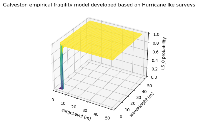
# use utility method of pyicore-viz package to visualize the fragility
fragility_set = FragilityCurveSet(FragilityService(client).get_dfr3_set("5f6ccf67de7b566bb71b202d"))
plt = plotviz.get_fragility_plot_3d(fragility_set,
                                            title="Galveston empirical fragility model developed "
                                            "based on Hurricane Ike surveys",
                                            limit_state="LS_0")
plt.show()
hazard_type = "hurricane"
# Galveston deterministic Hurricane, 3 datasets - Kriging
hazard_id = "5fa5a228b6429615aeea4410"

# visualization
wave_height_id = "5f15cd62c98cf43417c10a3f"
surge_level_id = "5f15cd5ec98cf43417c10a3b"

# Hurricane building mapping (with equation)
mapping_id = "602c381a1d85547cdc9f0675"
fragility_service = FragilityService(client)
mapping_set = MappingSet(fragility_service.get_mapping(mapping_id))

# Building Wind Fragility mapping
wind_mapping_id = "62fef3a6cef2881193f2261d"
wind_mapping_set = MappingSet(fragility_service.get_mapping(wind_mapping_id))

# Surge-wave mapping
sw_mapping_id = "6303e51bd76c6d0e1f6be080"
sw_mapping_set = MappingSet(fragility_service.get_mapping(sw_mapping_id))

# flood mapping
flood_mapping_id = "62fefd688a30d30dac57bbd7"
flood_mapping_set = MappingSet(fragility_service.get_mapping(flood_mapping_id))
# visualize wave height
dataset = Dataset.from_data_service(wave_height_id, DataService(client))
map = geoviz.map_raster_overlay_from_file(dataset.get_file_path('tif'))
map
Dataset already exists locally. Reading from local cached zip.
Unzipped folder found in the local cache. Reading from it...
# add opacity control - NOTE: It takes time before the opacity takes effect.
map.layers[1].interact(opacity=(0.0,1.0,0.01))
# visualize surge level
dataset = Dataset.from_data_service(surge_level_id, DataService(client))
map = geoviz.map_raster_overlay_from_file(dataset.get_file_path('tif'))
map
Dataset already exists locally. Reading from local cached zip.
Unzipped folder found in the local cache. Reading from it...
# add opacity control - NOTE: It takes time before the opacity takes effect.
map.layers[1].interact(opacity=(0.0,1.0,0.01))
2.2 Building Damage#
2.2.1 Wind building damage#
# wind building damage
w_bldg_dmg = BuildingDamage(client)
w_bldg_dmg.load_remote_input_dataset("buildings", bldg_dataset_id)
w_bldg_dmg.set_input_dataset('dfr3_mapping_set', wind_mapping_set)
w_bldg_dmg.set_parameter("result_name", "Galveston-wind-dmg")
w_bldg_dmg.set_parameter("hazard_type", hazard_type)
w_bldg_dmg.set_parameter("hazard_id", hazard_id)
w_bldg_dmg.set_parameter("num_cpu", 4)
w_bldg_dmg.run_analysis()
Dataset already exists locally. Reading from local cached zip.
Unzipped folder found in the local cache. Reading from it...
True
2.2.2 Surge-Wave building damage#
# surge-wave building damage
bldg_dmg = BuildingDamage(client)
bldg_dmg.load_remote_input_dataset("buildings", bldg_dataset_id)
bldg_dmg.set_input_dataset('dfr3_mapping_set', sw_mapping_set)
bldg_dmg.set_parameter("result_name", "Galveston-sw-dmg")
bldg_dmg.set_parameter("hazard_type", hazard_type)
bldg_dmg.set_parameter("hazard_id", hazard_id)
bldg_dmg.set_parameter("num_cpu", 4)
bldg_dmg.run_analysis()
Dataset already exists locally. Reading from local cached zip.
Unzipped folder found in the local cache. Reading from it...
True
Flood building damage#
# flood building damage
f_bldg_dmg = BuildingDamage(client)
f_bldg_dmg.load_remote_input_dataset("buildings", bldg_dataset_id)
f_bldg_dmg.set_input_dataset('dfr3_mapping_set', flood_mapping_set)
f_bldg_dmg.set_parameter("result_name", "Galveston-flood-dmg")
f_bldg_dmg.set_parameter("hazard_type", hazard_type)
f_bldg_dmg.set_parameter("hazard_id", hazard_id)
f_bldg_dmg.set_parameter("num_cpu", 4)
f_bldg_dmg.run_analysis()
Dataset already exists locally. Reading from local cached zip.
Unzipped folder found in the local cache. Reading from it...
True
Combine wind, wave and surge building damage#
surge_wave_damage = bldg_dmg.get_output_dataset("ds_result")
wind_damage = w_bldg_dmg.get_output_dataset("ds_result")
flood_damage = f_bldg_dmg.get_output_dataset("ds_result")

result_name = "Galveston-combined-dmg"
combined_bldg_dmg = CombinedWindWaveSurgeBuildingDamage(client)
combined_bldg_dmg.set_input_dataset("surge_wave_damage", surge_wave_damage)
combined_bldg_dmg.set_input_dataset("wind_damage", wind_damage)
combined_bldg_dmg.set_input_dataset("flood_damage", flood_damage)
combined_bldg_dmg.set_parameter("result_name", result_name)
# combined_bldg_dmg.run_analysis()

# combined_dmg = combined_bldg_dmg.get_output_dataset("result")
# combined_dmg_df = combined_dmg.get_dataframe_from_csv(low_memory=False)

# Display top 5 rows of output data
# combined_dmg_df.head()
True
2.3 Electric Power Facility Damage#
# EPF fragility mapping
epf_mapping_id = "62fac92ecef2881193f22613"
epf_mapping_set = MappingSet(fragility_service.get_mapping(epf_mapping_id))

epf_dmg_hurricane_galveston = EpfDamage(client)
epf_dmg_hurricane_galveston.load_remote_input_dataset("epfs", "62fc000f88470b319561b58d")
epf_dmg_hurricane_galveston.set_input_dataset('dfr3_mapping_set', epf_mapping_set)
epf_dmg_hurricane_galveston.set_parameter("result_name", "Galveston-hurricane-epf-damage")
epf_dmg_hurricane_galveston.set_parameter("fragility_key", "Non-Retrofit Fragility ID Code")
epf_dmg_hurricane_galveston.set_parameter("hazard_type", hazard_type)
epf_dmg_hurricane_galveston.set_parameter("hazard_id", hazard_id)
epf_dmg_hurricane_galveston.set_parameter("num_cpu", 8)

# Run Analysis
epf_dmg_hurricane_galveston.run_analysis()
---------------------------------------------------------------------------
NameError                                 Traceback (most recent call last)
Cell In[22], line 3
      1 # EPF fragility mapping
      2 epf_mapping_id = "62fac92ecef2881193f22613"
----> 3 epf_mapping_set = MappingSet(fragility_service.get_mapping(epf_mapping_id))
      5 epf_dmg_hurricane_galveston = EpfDamage(client)
      6 epf_dmg_hurricane_galveston.load_remote_input_dataset("epfs", "62fc000f88470b319561b58d")

NameError: name 'fragility_service' is not defined
3) Functionality#
3a) Functionality Models#

3b) Functionality of Physical Infrastructure#
# Retrieve result dataset from surge_wave_damage
building_dmg_result = bldg_dmg.get_output_dataset('ds_result')
# Convert dataset to Pandas DataFrame
bdmg_df = building_dmg_result.get_dataframe_from_csv(low_memory=False)

# Display top 5 rows of output data
bdmg_df.head()
| guid | LS_0 | LS_1 | LS_2 | DS_0 | DS_1 | DS_2 | DS_3 | haz_expose | |
|---|---|---|---|---|---|---|---|---|---|
| 0 | 1815653a-7b70-44ce-8544-e975596bdf82 | 0.0 | 0.0 | 0.0 | 1.0 | 0.0 | 0.0 | 0.0 | no |
| 1 | df63f574-8e9b-426b-aa3b-b3757cb699b5 | 0.0 | 0.0 | 0.0 | 1.0 | 0.0 | 0.0 | 0.0 | no |
| 2 | a743ae24-4209-44e2-b11e-7a872f071ae9 | 0.0 | 0.0 | 0.0 | 1.0 | 0.0 | 0.0 | 0.0 | no |
| 3 | 59ed0339-c8e3-4fcd-9b5a-c1487b035d3b | 0.0 | 0.0 | 0.0 | 1.0 | 0.0 | 0.0 | 0.0 | no |
| 4 | 5cc8a749-21ca-4073-8626-4ae7332cc0dd | 0.0 | 0.0 | 0.0 | 1.0 | 0.0 | 0.0 | 0.0 | no |
bdmg_df.DS_0.describe()
count    1.616450e+05
mean     9.034213e-01
std      2.621947e-01
min      3.279000e-07
25%      1.000000e+00
50%      1.000000e+00
75%      1.000000e+00
max      1.000000e+00
Name: DS_0, dtype: float64
bdmg_df.DS_3.describe()
count    161645.000000
mean          0.015951
std           0.110204
min           0.000000
25%           0.000000
50%           0.000000
75%           0.000000
max           0.999997
Name: DS_3, dtype: float64
4) Recovery#

j is the index for time
m is the community lifetime
K is the index for policy levers and decision combinations (PD)
4.1 Household-Level Housing Recovery Analysis#
The Household-Level Housing Recovery (HHHR) model developed by Sutley and Hamideh (2020) is used to simulate the housing recovery process of dislocated households.
The computation operates by segregating household units into five zones as a way of assigning social vulnerability. Then, using this vulnerability in conjunction with the Transition Probability Matrix (TPM) and the initial state vector, a Markov chain computation simulates the most probable states to generate a stage history of housing recovery changes for each household. The detailed process of the HHHR model can be found in Sutley and Hamideh (2020).
Sutley, E.J. and Hamideh, S., 2020. Postdisaster housing stages: a Markov chain approach to model sequences and duration based on social vulnerability. Risk Analysis, 40(12), pp.2675-2695.
The Markov chain model consists of five discrete states at any time throughout the housing recovery process. The five discrete states represent stages in the household housing recovery process, including emergency shelter (1), temporary shelter (2); temporary housing (3); permanent housing (4), and failure to recover (5). The model assumes that a household can be in any of the first four stages immediately after a disaster. If the household reported not being dislocated, household will begin in stage 4.
4.2 Set Up and Run Household-level Housing Sequential Recovery#
# Parameters
state = "texas"
county = "galveston"
year = 2020
# get fips code to use fetch census data
fips = CensusUtil.get_fips_by_state_county(state=state, county=county)
state_code = fips[:2]
county_code = fips[2:]
def demographic_factors(state_number, county_number, year, geo_type="tract:*"):
_, df_1 = CensusUtil.get_census_data(state=state_code, county=county_code, year=year,
data_source="acs/acs5",
columns="GEO_ID,B03002_001E,B03002_003E",
geo_type=geo_type)
df_1["factor_white_nonHispanic"] = df_1[["B03002_001E","B03002_003E"]].astype(int).apply(lambda row: row["B03002_003E"]/row["B03002_001E"], axis = 1)
_, df_2 = CensusUtil.get_census_data(state=state_code, county=county_code, year=year,
data_source="acs/acs5",
columns="B25003_001E,B25003_002E",
geo_type=geo_type)
df_2["factor_owner_occupied"] = df_2.astype(int).apply(lambda row: row["B25003_002E"]/row["B25003_001E"], axis = 1)
_, df_3 = CensusUtil.get_census_data(state=state_code,
county=county_code,
year=year,
data_source="acs/acs5",
columns="B17021_001E,B17021_002E",
geo_type=geo_type)
df_3["factor_earning_higher_than_national_poverty_rate"] = df_3.astype(int).apply(lambda row: 1-row["B17021_002E"]/row["B17021_001E"], axis = 1)
_, df_4 = CensusUtil.get_census_data(state=state_code,
county=county_code,
year=year,
data_source="acs/acs5",
columns="B15003_001E,B15003_017E,B15003_018E,B15003_019E,B15003_020E,B15003_021E,B15003_022E,B15003_023E,B15003_024E,B15003_025E",
geo_type=geo_type)
df_4["factor_over_25_with_high_school_diploma_or_higher"] = df_4.astype(int).apply(lambda row: (row["B15003_017E"]
+ row["B15003_018E"]
+ row["B15003_019E"]
+ row["B15003_020E"]
+ row["B15003_021E"]
+ row["B15003_022E"]
+ row["B15003_023E"]
+ row["B15003_024E"]
+ row["B15003_025E"])/row["B15003_001E"], axis = 1)
if geo_type == 'tract:*':
_, df_5 = CensusUtil.get_census_data(state=state_code,
county=county_code,
year=year,
data_source="acs/acs5",
columns="B18101_001E,B18101_011E,B18101_014E,B18101_030E,B18101_033E",
geo_type=geo_type)
df_5["factor_without_disability_age_18_to_65"] = df_5.astype(int).apply(lambda row: (row["B18101_011E"] + row["B18101_014E"] + row["B18101_030E"] + row["B18101_033E"])/row["B18101_001E"], axis = 1)
elif geo_type == 'block%20group:*':
_, df_5 = CensusUtil.get_census_data(state=state_code,
county=county_code,
year=year,
data_source="acs/acs5",
columns="B01003_001E,C21007_006E,C21007_009E,C21007_013E,C21007_016E",
geo_type=geo_type)
df_5['factor_without_disability_age_18_to_65'] = df_5.astype(int).apply(lambda row: (row['C21007_006E']+
row['C21007_006E']+
row['C21007_009E']+
row['C21007_013E'])
/row['C21007_016E'], axis = 1)
df_t = pd.concat([df_1[["GEO_ID","factor_white_nonHispanic"]],
df_2["factor_owner_occupied"],
df_3["factor_earning_higher_than_national_poverty_rate"],
df_4["factor_over_25_with_high_school_diploma_or_higher"],
df_5["factor_without_disability_age_18_to_65"]],
axis=1, join='inner')
# extract FIPS from geo id
df_t["FIPS"] = df_t.apply(lambda row: row["GEO_ID"].split("US")[1], axis = 1)
return df_t
def national_ave_values(year, data_source="acs/acs5"):
_, nav1 = CensusUtil.get_census_data(state="*", county=None, year=year, data_source=data_source,
columns="B03002_001E,B03002_003E",geo_type=None)
nav1 = nav1.astype(int)
nav1_avg ={"feature": "NAV-1: White, nonHispanic",
"average": nav1['B03002_003E'].sum()/ nav1['B03002_001E'].sum()}
_, nav2 = CensusUtil.get_census_data(state="*", county=None, year=year, data_source=data_source,
columns="B25003_001E,B25003_002E",geo_type=None)
nav2 = nav2.astype(int)
nav2_avg = {"feature": "NAV-2: Home Owners",
"average": nav2['B25003_002E'].sum()/nav2['B25003_001E'].sum()}
_, nav3 = CensusUtil.get_census_data(state="*", county=None, year=year, data_source=data_source,
columns="B17021_001E,B17021_002E",geo_type=None)
nav3 = nav3.astype(int)
nav3_avg = {"feature": "NAV-3: earning higher than national poverty rate",
"average": 1-nav3['B17021_002E'].sum()/nav3['B17021_001E'].sum()}
_, nav4 = CensusUtil.get_census_data(state="*",
county=None,
year=year,
data_source="acs/acs5",
columns="B15003_001E,B15003_017E,B15003_018E,B15003_019E,B15003_020E,B15003_021E,B15003_022E,B15003_023E,B15003_024E,B15003_025E",
geo_type=None)
nav4 = nav4.astype(int)
nav4['temp'] = nav4.apply(lambda row: row['B15003_017E']+row['B15003_018E']+row['B15003_019E']+
row['B15003_020E']+row['B15003_021E']+row['B15003_022E']+row['B15003_023E']+
row['B15003_024E']+row['B15003_025E'], axis = 1)
nav4_avg = {"feature": 'NAV-4: over 25 with high school diploma or higher',
"average": nav4['temp'].sum()/nav4['B15003_001E'].sum()}
_, nav5 = CensusUtil.get_census_data(state="*", county=None, year=year, data_source=data_source,
columns="B18101_001E,B18101_011E,B18101_014E,B18101_030E,B18101_033E",
geo_type=None)
nav5 = nav5.astype(int)
nav5['temp'] = nav5.apply(lambda row: row['B18101_011E']+row['B18101_014E']+row['B18101_030E']+row['B18101_033E'], axis = 1)
nav5_avg = {"feature": 'NAV-5: without disability age 18 to 65',
"average": nav5["temp"].sum()/nav5["B18101_001E"].sum()}
navs = [nav1_avg, nav2_avg, nav3_avg, nav4_avg, nav5_avg]
return navs
navs = national_ave_values(year=year)
national_vulnerability_feature_averages = Dataset.from_csv_data(navs, name="national_vulnerability_feature_averages.csv",
data_type="incore:socialVulnerabilityFeatureAverages")
geo_type = "block%20group:*"
# geo_type = "tract:*"
social_vunlnerability_dem_factors_df = demographic_factors(state_code, county_code, year=year, geo_type=geo_type)
# Temp fix: remove bad data point
social_vunlnerability_dem_factors_df = social_vunlnerability_dem_factors_df.dropna()
social_vunlnerability_dem_factors = Dataset.from_dataframe(social_vunlnerability_dem_factors_df,
name="social_vunlnerability_dem_factors",
data_type="incore:socialVulnerabilityDemFactors")
social_vulnerability = SocialVulnerability(client)
social_vulnerability.set_parameter("result_name", "social_vulnerabilty")
social_vulnerability.set_input_dataset("national_vulnerability_feature_averages", national_vulnerability_feature_averages)
social_vulnerability.set_input_dataset("social_vulnerability_demographic_factors", social_vunlnerability_dem_factors)
True
# Run social vulnerability damage analysis
result = social_vulnerability.run_analysis()
# Retrieve result dataset
sv_result = social_vulnerability.get_output_dataset("sv_result")
# Convert dataset to Pandas DataFrame
df = sv_result.get_dataframe_from_csv()
# Display top 5 rows of output data
df.head()
| GEO_ID | factor_white_nonHispanic | factor_owner_occupied | factor_earning_higher_than_national_poverty_rate | factor_over_25_with_high_school_diploma_or_higher | factor_without_disability_age_18_to_65 | FIPS | R1 | R2 | R3 | R4 | R5 | SVS | zone | |
|---|---|---|---|---|---|---|---|---|---|---|---|---|---|---|
| 0 | 1500000US481677201001 | 0.826873 | 0.857143 | 0.836348 | 0.985014 | 0.075404 | 481677201001 | 1.389439 | 1.330196 | 0.962965 | 1.114087 | 0.137041 | 0.986746 | Medium Vulnerable (zone3) |
| 1 | 1500000US481677201002 | 0.676741 | 0.889262 | 0.894875 | 0.929273 | 0.176230 | 481677201002 | 1.137164 | 1.380041 | 1.030353 | 1.051042 | 0.320285 | 0.983777 | Medium Vulnerable (zone3) |
| 2 | 1500000US481677201003 | 0.517323 | 0.809955 | 0.984252 | 0.980989 | 0.056364 | 481677201003 | 0.869285 | 1.256965 | 1.133261 | 1.109534 | 0.102437 | 0.894296 | Medium to High Vulnerable (zone4) |
| 3 | 1500000US481677201004 | 0.561679 | 1.000000 | 1.000000 | 0.919908 | 0.061051 | 481677201004 | 0.943819 | 1.551895 | 1.151393 | 1.040451 | 0.110956 | 0.959703 | Medium Vulnerable (zone3) |
| 4 | 1500000US481677202001 | 0.701548 | 0.973113 | 0.987214 | 0.973601 | 0.062718 | 481677202001 | 1.178848 | 1.510169 | 1.136671 | 1.101179 | 0.113985 | 1.008170 | Medium Vulnerable (zone3) |
# Transition probability matrix per social vulnerability level, from Sutley and Hamideh (2020).
transition_probability_matrix = "60f5e2ae544e944c3cec0794"
# Initial mass probability function for household at time 0
initial_probability_vector = "60f5e918544e944c3cec668b"
# Create housing recovery instance
housing_recovery = HousingRecoverySequential(client)
# Load input datasets from dislocation, tpm, and initial probability function
#housing_recovery.load_remote_input_dataset("population_dislocation_block", population_dislocation)
housing_recovery.set_input_dataset("population_dislocation_block", population_dislocation_result)
housing_recovery.load_remote_input_dataset("tpm", transition_probability_matrix)
housing_recovery.load_remote_input_dataset("initial_stage_probabilities", initial_probability_vector)
Dataset already exists locally. Reading from local cached zip.
Unzipped folder found in the local cache. Reading from it...
Dataset already exists locally. Reading from local cached zip.
Unzipped folder found in the local cache. Reading from it...
# Initial value to seed the random number generator to ensure replication
seed = 1234
# A size of the analysis time step in month
t_delta = 1.0
# Total duration of Markov chain recovery process
t_final = 90.0
# Specify the result name
result_name = "housing_recovery_result"

# Set analysis parameters
housing_recovery.set_parameter("result_name", result_name)
housing_recovery.set_parameter("seed", seed)
housing_recovery.set_parameter("t_delta", t_delta)
housing_recovery.set_parameter("t_final", t_final)

# Chain with SV output
housing_recovery.set_input_dataset('sv_result', sv_result)

# Run the household recovery sequence analysis - Markov model
housing_recovery.run()
6 a) Sufficient Quality Solutions Found?#
# Retrieve result dataset
housing_recovery_result = housing_recovery.get_output_dataset("ds_result")

# Convert dataset to Pandas DataFrame
df_hhrs = housing_recovery_result.get_dataframe_from_csv()

# Display top 5 rows of output data
df_hhrs.head()
| guid | huid | Zone | SV | 1 | 2 | 3 | 4 | 5 | 6 | ... | 81 | 82 | 83 | 84 | 85 | 86 | 87 | 88 | 89 | 90 | |
|---|---|---|---|---|---|---|---|---|---|---|---|---|---|---|---|---|---|---|---|---|---|
| 0 | df7e5aef-c49f-45dd-b145-6fd7db8f50ff | B481677201001000H222 | Z3 | 0.524 | 4.0 | 4.0 | 4.0 | 4.0 | 4.0 | 4.0 | ... | 4.0 | 4.0 | 4.0 | 4.0 | 4.0 | 4.0 | 4.0 | 4.0 | 4.0 | 4.0 |
| 1 | 07b29b24-3184-4d0b-bbc6-1538aee5b1f1 | B481677201001000H076 | Z3 | 0.557 | 4.0 | 4.0 | 4.0 | 4.0 | 4.0 | 4.0 | ... | 4.0 | 4.0 | 4.0 | 4.0 | 4.0 | 4.0 | 4.0 | 4.0 | 4.0 | 4.0 |
| 2 | 6d9c5304-59ff-4fb4-a8cf-d746b98f95fb | B481677201001000H160 | Z3 | 0.455 | 4.0 | 4.0 | 4.0 | 4.0 | 4.0 | 4.0 | ... | 4.0 | 4.0 | 4.0 | 4.0 | 4.0 | 4.0 | 4.0 | 4.0 | 4.0 | 4.0 |
| 3 | 2f76cc1d-ee76-445c-b086-2cd331ed7b1b | B481677201001000H084 | Z3 | 0.560 | 4.0 | 4.0 | 4.0 | 4.0 | 4.0 | 4.0 | ... | 4.0 | 4.0 | 4.0 | 4.0 | 4.0 | 4.0 | 4.0 | 4.0 | 4.0 | 4.0 |
| 4 | cdcedef2-2948-459f-b453-3fcc19076d91 | B481677201001000H182 | Z3 | 0.950 | 4.0 | 4.0 | 4.0 | 4.0 | 4.0 | 4.0 | ... | 4.0 | 4.0 | 4.0 | 4.0 | 4.0 | 4.0 | 4.0 | 4.0 | 4.0 | 4.0 |
5 rows × 94 columns
Explore Household-level Housing Recovery Results#
df_hhrs['1'].describe()
count    77398.000000
mean         3.702861
std          0.890408
min          1.000000
25%          4.000000
50%          4.000000
75%          4.000000
max          4.000000
Name: 1, dtype: float64
# Locate observations where timestep 1 does not equal 4
df_hhrs[df_hhrs['13'] != 4].head()
| guid | huid | Zone | SV | 1 | 2 | 3 | 4 | 5 | 6 | ... | 81 | 82 | 83 | 84 | 85 | 86 | 87 | 88 | 89 | 90 | |
|---|---|---|---|---|---|---|---|---|---|---|---|---|---|---|---|---|---|---|---|---|---|
| 14327 | 840a174d-fe0b-4e7f-9490-de70e6972268 | B481677210001005H011 | Z4 | 0.655 | 1.0 | 2.0 | 3.0 | 2.0 | 3.0 | 2.0 | ... | 4.0 | 4.0 | 4.0 | 4.0 | 4.0 | 4.0 | 4.0 | 4.0 | 4.0 | 4.0 |
| 14339 | 7e852dc1-e2f3-454c-96fb-024f80f3d36c | B481677210001005H012 | Z4 | 0.827 | 1.0 | 1.0 | 1.0 | 1.0 | 1.0 | 1.0 | ... | 4.0 | 4.0 | 4.0 | 4.0 | 4.0 | 4.0 | 4.0 | 4.0 | 4.0 | 4.0 |
| 14343 | 6d6d79b3-50b0-43f8-a5fa-15a0ab91e30d | B481677210001007H012 | Z4 | 0.799 | 2.0 | 2.0 | 1.0 | 2.0 | 1.0 | 2.0 | ... | 4.0 | 4.0 | 4.0 | 4.0 | 4.0 | 4.0 | 4.0 | 4.0 | 4.0 | 4.0 |
| 14363 | e9d5a4ed-5356-4674-af60-7165c29a1e3f | B481677210001007H017 | Z4 | 0.674 | 2.0 | 2.0 | 2.0 | 2.0 | 2.0 | 2.0 | ... | 4.0 | 4.0 | 4.0 | 4.0 | 4.0 | 4.0 | 4.0 | 4.0 | 4.0 | 4.0 |
| 14369 | 61c09dbe-5099-4dc5-8b94-87750fe340a3 | B481677210001007H053 | Z4 | 0.760 | 1.0 | 1.0 | 2.0 | 3.0 | 3.0 | 2.0 | ... | 4.0 | 4.0 | 4.0 | 4.0 | 4.0 | 4.0 | 4.0 | 4.0 | 4.0 | 4.0 |
5 rows × 94 columns
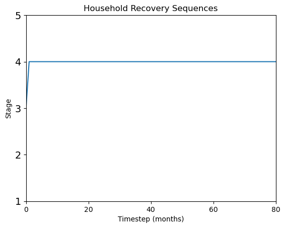
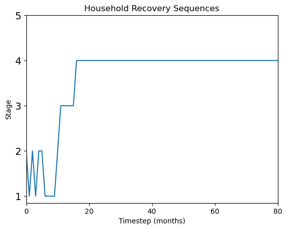
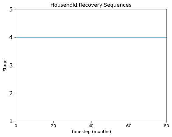
Plot Housing Recovery Sequence Results
view recovery sequence results for specific households
df=df_hhrs.drop(['guid', 'huid', 'Zone', 'SV'], axis=1).copy()
df=df.to_numpy()
t_steps=int(t_final)-1

# Plot stage histories and stage changes using pandas.
# Generate timestep labels for dataframes.
label_timestep = []
for i4 in range(0, t_steps):
    label_timestep.append(str(i4))

ids = [9700,14343,48] # select specific household by id numbers
for id in ids:
    HH_stagehistory_DF = pd.DataFrame(np.transpose(df[id, 1:]),
                                      index=label_timestep)
    ax = HH_stagehistory_DF.reset_index().plot(x='index',
                                               yticks=[1, 2, 3, 4, 5],
                                               title='Household Recovery Sequences',
                                               legend=False)
    ax.set(xlabel='Timestep (months)', ylabel='Stage')
    y_ticks_labels = ['1','2','3','4','5']
    ax.set_xlim(0,80)
    ax.set_yticklabels(y_ticks_labels, fontsize = 14)
Plot recovery heatmap any stage of recovery
df_hhrs.head()
| guid | huid | Zone | SV | 1 | 2 | 3 | 4 | 5 | 6 | ... | 81 | 82 | 83 | 84 | 85 | 86 | 87 | 88 | 89 | 90 | |
|---|---|---|---|---|---|---|---|---|---|---|---|---|---|---|---|---|---|---|---|---|---|
| 0 | df7e5aef-c49f-45dd-b145-6fd7db8f50ff | B481677201001000H222 | Z3 | 0.524 | 4.0 | 4.0 | 4.0 | 4.0 | 4.0 | 4.0 | ... | 4.0 | 4.0 | 4.0 | 4.0 | 4.0 | 4.0 | 4.0 | 4.0 | 4.0 | 4.0 |
| 1 | 07b29b24-3184-4d0b-bbc6-1538aee5b1f1 | B481677201001000H076 | Z3 | 0.557 | 4.0 | 4.0 | 4.0 | 4.0 | 4.0 | 4.0 | ... | 4.0 | 4.0 | 4.0 | 4.0 | 4.0 | 4.0 | 4.0 | 4.0 | 4.0 | 4.0 |
| 2 | 6d9c5304-59ff-4fb4-a8cf-d746b98f95fb | B481677201001000H160 | Z3 | 0.455 | 4.0 | 4.0 | 4.0 | 4.0 | 4.0 | 4.0 | ... | 4.0 | 4.0 | 4.0 | 4.0 | 4.0 | 4.0 | 4.0 | 4.0 | 4.0 | 4.0 |
| 3 | 2f76cc1d-ee76-445c-b086-2cd331ed7b1b | B481677201001000H084 | Z3 | 0.560 | 4.0 | 4.0 | 4.0 | 4.0 | 4.0 | 4.0 | ... | 4.0 | 4.0 | 4.0 | 4.0 | 4.0 | 4.0 | 4.0 | 4.0 | 4.0 | 4.0 |
| 4 | cdcedef2-2948-459f-b453-3fcc19076d91 | B481677201001000H182 | Z3 | 0.950 | 4.0 | 4.0 | 4.0 | 4.0 | 4.0 | 4.0 | ... | 4.0 | 4.0 | 4.0 | 4.0 | 4.0 | 4.0 | 4.0 | 4.0 | 4.0 | 4.0 |
5 rows × 94 columns
# Keep housing units for Galveston Island
pd_df_community = pd_df.loc[pd_df['placeNAME10']=='Galveston'].copy()
pd_df_community['placeNAME10'].describe()
count         32128
unique            1
top       Galveston
freq          32128
Name: placeNAME10, dtype: object
# merge household unit information with recovery results
pd_df_hs = pd.merge(left = pd_df_community,
                    right = df_hhrs,
                    left_on=['guid','huid'],
                    right_on=['guid','huid'],
                    how='left')
pd_df_hs[['guid','huid']].describe()
| guid | huid | |
|---|---|---|
| count | 32128 | 32128 |
| unique | 19983 | 32128 |
| top | 2669f722-ae95-4181-90a8-9c4755b7b29c | B481677240001010H034 |
| freq | 191 | 1 |
Create recovery curve based on income groups#
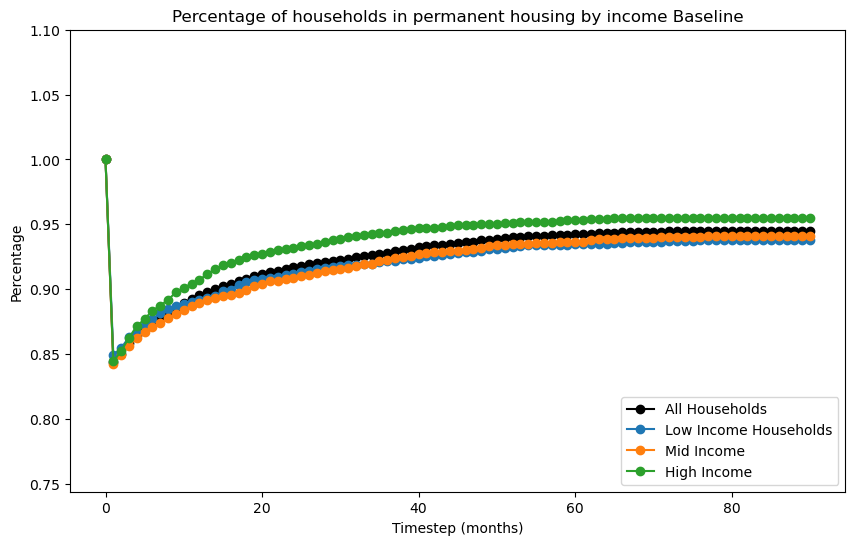
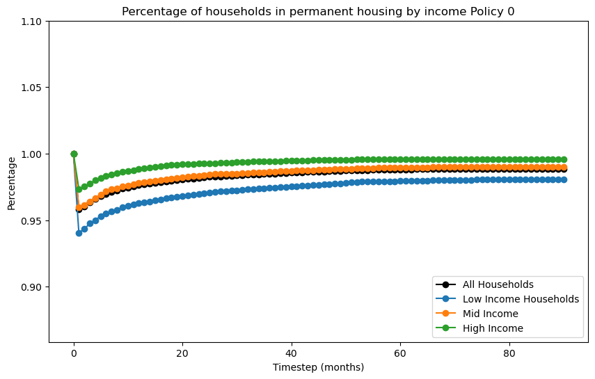
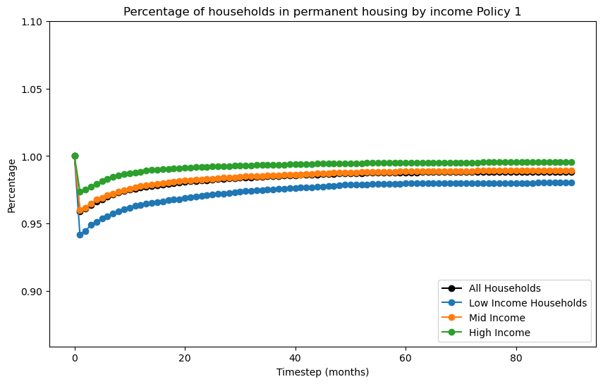
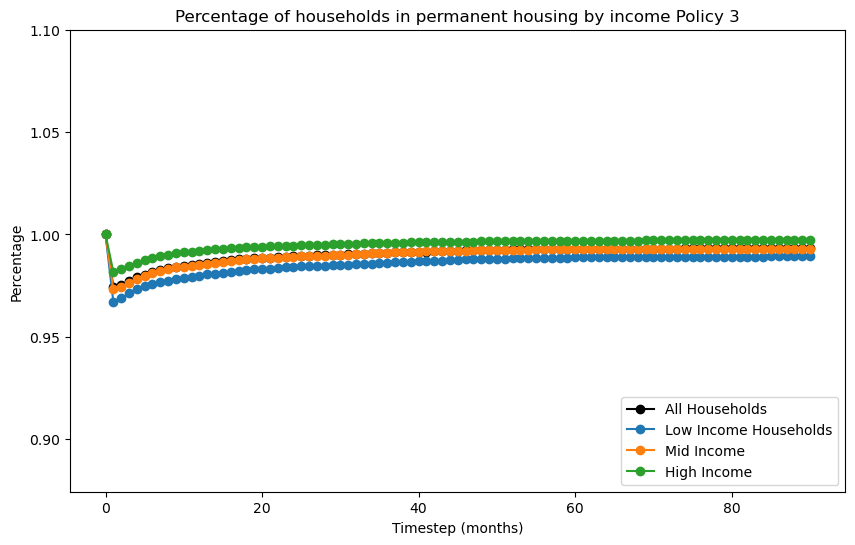
Code will loop through data over time to create percent in permanent housing at each time step.
def recovery_curve_byincome(pd_df_hs,
                            filename,
                            subtitle : str = ""):
    """
    Generate a recovery curve based on building damage, population dislocation,
    and household housing recovery model.

    """
    total_housingunits = pd_df_hs.shape[0]
    total_households = pd_df_hs.loc[(pd_df_hs['randincome'].notnull())].shape[0]
    #print("Total housing units:", total_housingunits)
    #print("Total households:", total_households)

    # What is the distribution of housing units by income?
    pd_df_hs['income_quantile'] = pd.qcut(pd_df_hs['randincome'], 5, labels=False)
    #pd_df_hs[['randincome','income_quantile']].groupby('income_quantile').describe()

    total_lowincomehouseholds = pd_df_hs.loc[(pd_df_hs['income_quantile'] == 0)].shape[0]
    total_midincomehouseholds = pd_df_hs.loc[(pd_df_hs['income_quantile'] == 2)].shape[0]
    total_highincomehouseholds = pd_df_hs.loc[(pd_df_hs['income_quantile'] == 4)].shape[0]
    #print("Total low income households:", total_lowincomehouseholds)
    #print("Total mid income households:", total_midincomehouseholds)
    #print("Total high income households:", total_highincomehouseholds)

    # loop over variables 1 to 90
    dict = {}
    # Create dataframe to store values
    # Assume at time 0, all households are in permanent housing
    dict[str(0)] = pd.DataFrame([{'timestep' : 0,
                    'total_households' : total_housingunits,
                    'notperm': 0,
                    'total_highincomehouseholds': total_highincomehouseholds,
                    'total_midincomehouseholds': total_midincomehouseholds,
                    'total_lowincomehouseholds': total_lowincomehouseholds,
                    'lowincome_notperm': 0,
                    'midincome_notperm': 0,
                    'highincome_notperm': 0}])

    for i in range(1,91):
        # create dictionary entry that summarizes the number of households not in permanent housing
        households_notinpermanthousing = pd_df_hs.loc[(pd_df_hs[str(i)] != 4) &
                                                    (pd_df_hs[str(i)].notnull()) &
                                                    (pd_df_hs['randincome'].notnull())].shape[0]
        lowincome_households_notinpermanthousing = pd_df_hs.loc[(pd_df_hs[str(i)] != 4) &
                                                    (pd_df_hs[str(i)].notnull()) &
                                                    (pd_df_hs['income_quantile'] == 0)].shape[0]
        midincome_households_notinpermanthousing = pd_df_hs.loc[(pd_df_hs[str(i)] != 4) &
                                                    (pd_df_hs[str(i)].notnull()) &
                                                    (pd_df_hs['income_quantile'] == 2)].shape[0]
        highincome_households_notinpermanthousing = pd_df_hs.loc[(pd_df_hs[str(i)] != 4) &
                                                    (pd_df_hs[str(i)].notnull()) &
                                                    (pd_df_hs['income_quantile'] == 4)].shape[0]

        # Create dataframe to store values
        dict[str(i)] = pd.DataFrame([{'timestep' : i,
                        'total_households' : total_households,
                        'notperm': households_notinpermanthousing,
                        'total_highincomehouseholds': total_highincomehouseholds,
                        'total_midincomehouseholds': total_midincomehouseholds,
                        'total_lowincomehouseholds': total_lowincomehouseholds,
                        'lowincome_notperm': lowincome_households_notinpermanthousing,
                        'midincome_notperm': midincome_households_notinpermanthousing,
                        'highincome_notperm': highincome_households_notinpermanthousing}])

    # convert dictionary to dataframe
    df_summary = pd.concat(dict.values())
    df_summary['percent_allperm'] = 1 - (df_summary['notperm']/ \
                                        df_summary['total_households'] )
    df_summary['percent_lowperm'] = 1 - (df_summary['lowincome_notperm']/ \
                                    df_summary['total_lowincomehouseholds'] )
    df_summary['percent_midperm'] = 1 - (df_summary['midincome_notperm']/ \
                                        df_summary['total_midincomehouseholds'] )
    df_summary['percent_highperm'] = 1 - (df_summary['highincome_notperm']/ \
                                    df_summary['total_highincomehouseholds'] )

    # plot
    # Start new figure
    fig = plt.figure(figsize=(10,6))
    plt.plot('timestep', 'percent_allperm',
            data = df_summary,
            linestyle='-', marker='o', color='black')
    plt.plot('timestep', 'percent_lowperm',
            data = df_summary,
            linestyle='-', marker='o')
    plt.plot('timestep', 'percent_midperm',
            data = df_summary,
            linestyle='-', marker='o')
    plt.plot('timestep', 'percent_highperm',
            data = df_summary,
            linestyle='-', marker='o')
    # Set y-axis range
    # What is the minimum and maximum values of the percent of households in permanent housing?
    ylim_lower = df_summary['percent_allperm'].min()-.1
    ylim_upper = df_summary['percent_allperm'].max()+.1
    plt.ylim(ylim_lower,ylim_upper)
    # Relable legend
    plt.legend(['All Households','Low Income Households', 'Mid Income', 'High Income'],
                loc='lower right')
    # Add title
    plt.title('Percentage of households in permanent housing by income'+subtitle)
    # Add x and y labels
    plt.xlabel('Timestep (months)')
    plt.ylabel('Percentage')
    # save plot
    plt.savefig(f'{filename}.pdf', bbox_inches='tight', dpi = 1000)

    plt.show()
    # good practice to close the plt object.
    plt.close()
# Create container to store filenames (use to make a GIF)
# https://towardsdatascience.com/basics-of-gifs-with-pythons-matplotlib-54dd544b6f30
filenames = []
i = 0
recovery_curve_byincome(pd_df_hs = pd_df_hs,
                        filename = f'recovery_curve_byincome{i}',
                        subtitle=' Baseline')
filenames.append(filename)
Plot recovery heatmap after 12 months of recovery
from ipyleaflet import Map, Heatmap, LayersControl, LegendControl

# What location should the map be centered on?
center_x = pd_df_hs['x'].mean()
center_y = pd_df_hs['y'].mean()

map = Map(center=[center_y, center_x], zoom=11)

stage5_data = pd_df_hs[['y','x','numprec']].loc[pd_df_hs['85']==5].values.tolist()
stage5 = Heatmap(
    locations = stage5_data,
    radius = 5,
    max_val = 1000,
    blur = 10,
    gradient={0.2: 'yellow', 0.5: 'orange', 1.0: 'red'},
    name = 'Stage 5 - Failure to Recover',
)

stage4_data = pd_df_hs[['y','x','numprec']].loc[pd_df_hs['85']==4].values.tolist()
stage4 = Heatmap(
    locations = stage4_data,
    radius = 5,
    max_val = 1000,
    blur = 10,
    gradient={0.2: 'purple', 0.5: 'blue', 1.0: 'green'},
    name = 'Stage 4 - Permanent Housing',
)

map.add_layer(stage4)
map.add_layer(stage5)


control = LayersControl(position='topright')
map.add_control(control)
map
The five discrete states represent stages in the household housing recovery process, including emergency shelter (1), temporary shelter (2); temporary housing (3); permanent housing (4), and failure to recover (5). The model assumes that a household can be in any of the first four stages immediately after a disaster.
hhrs_valuelabels = {'categorical_variable' : {'variable' : 'select time step',
                   'variable_label' : 'Household housing recovery stages',
                   'notes' : 'Sutley and Hamideh recovery stages'},
              'value_list' : {
                1 : {'value': 1, 'value_label': "1 Emergency Shelter"},
                2 : {'value': 2, 'value_label': "2 Temporary Shelter"},
                3 : {'value': 3, 'value_label': "3 Temporary Housing"},
                4 : {'value': 4, 'value_label': "4 Permanent Housing"},
                5 : {'value': 5, 'value_label': "5 Failure to Recover"}}
            }

permanenthousing_valuelabels = {'categorical_variable' : {'variable' : 'select time step',
                   'variable_label' : 'Permanent Housing',
                   'notes' : 'Sutley and Hamideh recovery stages'},
              'value_list' : {
                1 : {'value': 1, 'value_label': "0 Not Permanent Housing"},
                2 : {'value': 2, 'value_label': "0 Not Permanent Housing"},
                3 : {'value': 3, 'value_label': "0 Not Permanent Housing"},
                4 : {'value': 4, 'value_label': "1 Permanent Housing"},
                5 : {'value': 5, 'value_label': "0 Not Permanent Housing"}}
            }

pd_df_hs = add_label_cat_values_df(pd_df_hs, valuelabels = hhrs_valuelabels, variable = '13')
pd_df_hs = add_label_cat_values_df(pd_df_hs, valuelabels = permanenthousing_valuelabels,
                        variable = '13')
poptable.pop_results_table(pd_df_hs.loc[(pd_df_hs['placeNAME10']=='Galveston')].copy(),
                  who = "Total Population by Householder",
                  what = "by Housing Type at T=13 by Race Ethnicity",
                  where = "Galveston Island TX",
                  when = "2010",
                  row_index = 'Race Ethnicity',
                  col_index = 'Household housing recovery stages',
                  row_percent = '2 Temporary Shelter'
                  )
| Household housing recovery stages | 1 Emergency Shelter (%) | 2 Temporary Shelter (%) | 3 Temporary Housing (%) | 4 Permanent Housing (%) | 5 Failure to Recover (%) | Total Population by Householder (%) | Percent Row 2 Temporary Shelter |
|---|---|---|---|---|---|---|---|
| Race Ethnicity | |||||||
| 1 White alone, Not Hispanic | 358 (50.2%) | 443 (50.7%) | 244 (55.5%) | 8,572 (52.3%) | 1 (25.0%) | 9,618 (52.2%) | 4.6% |
| 2 Black alone, Not Hispanic | 139 (19.5%) | 159 (18.2%) | 77 (17.5%) | 2,799 (17.1%) | 1 (25.0%) | 3,175 (17.2%) | 5.0% |
| 3 American Indian and Alaska Native alone, Not Hispanic | 6 (0.8%) | 3 (0.3%) | 2 (0.5%) | 68 (0.4%) | nan (nan%) | 79 (0.4%) | 3.8% |
| 4 Asian alone, Not Hispanic | 15 (2.1%) | 33 (3.8%) | 15 (3.4%) | 566 (3.5%) | nan (nan%) | 629 (3.4%) | 5.2% |
| 5 Other Race, Not Hispanic | 7 (1.0%) | 6 (0.7%) | 1 (0.2%) | 202 (1.2%) | nan (nan%) | 216 (1.2%) | 2.8% |
| 6 Any Race, Hispanic | 188 (26.4%) | 230 (26.3%) | 101 (23.0%) | 4,153 (25.3%) | 2 (50.0%) | 4,674 (25.4%) | 4.9% |
| 7 Group Quarters no Race Ethnicity Data | nan (nan%) | nan (nan%) | nan (nan%) | 26 (0.2%) | nan (nan%) | 26 (0.1%) | nan% |
| Total | 713 (100.0%) | 874 (100.0%) | 440 (100.0%) | 16,386 (100.0%) | 4 (100.0%) | 18,417 (100.0%) | 4.7% |
poptable.pop_results_table(pd_df_hs.loc[pd_df_hs['placeNAME10']=='Galveston'].copy(),
                  who = "Total Population by Householder",
                  what = "by Permanent Housing at T=13 by Race Ethnicity",
                  where = "Galveston Island TX",
                  when = "2010",
                  row_index = 'Race Ethnicity',
                  col_index = 'Permanent Housing',
                  row_percent = "0 Not Permanent Housing"
                  )
| Permanent Housing | 0 Not Permanent Housing (%) | 1 Permanent Housing (%) | Total Population by Householder (%) | Percent Row 0 Not Permanent Housing |
|---|---|---|---|---|
| Race Ethnicity | ||||
| 1 White alone, Not Hispanic | 1,046 (51.5%) | 8,572 (52.3%) | 9,618 (52.2%) | 10.9% |
| 2 Black alone, Not Hispanic | 376 (18.5%) | 2,799 (17.1%) | 3,175 (17.2%) | 11.8% |
| 3 American Indian and Alaska Native alone, Not Hispanic | 11 (0.5%) | 68 (0.4%) | 79 (0.4%) | 13.9% |
| 4 Asian alone, Not Hispanic | 63 (3.1%) | 566 (3.5%) | 629 (3.4%) | 10.0% |
| 5 Other Race, Not Hispanic | 14 (0.7%) | 202 (1.2%) | 216 (1.2%) | 6.5% |
| 6 Any Race, Hispanic | 521 (25.7%) | 4,153 (25.3%) | 4,674 (25.4%) | 11.1% |
| 7 Group Quarters no Race Ethnicity Data | nan (nan%) | 26 (0.2%) | 26 (0.1%) | nan% |
| Total | 2,031 (100.0%) | 16,386 (100.0%) | 18,417 (100.0%) | 11.0% |
8b) Policy Lever and Decision Combinations#
Hypothetical scenario to elevate all buildings in inventory.
# Create container to store filenames (use to make a GIF)
# https://towardsdatascience.com/basics-of-gifs-with-pythons-matplotlib-54dd544b6f30
recovery_curve_filenames = []
bldg_gdf_policy2 = bldg_df.copy()
#for i in range(18):
for i in range(4):

    ################## 1a) updated building inventory ##################
    print(f"Running Analysis: {i}")
    if i>0:
        bldg_gdf_policy2.loc[bldg_gdf_policy2['ffe_elev'].le(16), 'ffe_elev'] += 4
        #bldg_gdf_policy2.loc[bldg_gdf_policy2['lhsm_elev'].le(16), 'lhsm_elev'] += 1

        bldg_gdf_policy2.to_csv(f'input_df_{i}.csv')
    # Save new shapefile and then use as new input to building damage model
    bldg_gdf_policy2.to_file(driver = 'ESRI Shapefile', filename = f'bldg_gdf_policy_{i}.shp')
    # Plot and save
    #geoviz.plot_gdf_map(bldg_gdf_policy2, column='lhsm_elev',category='False')
    # Code to save the results here
    ####################################################################
    #
    #
    ################## 2c) Damage to Physical Infrastructure ##################
    building_inv_policy2 = Dataset.from_file(file_path = f'bldg_gdf_policy_{i}.shp',
                                        data_type='ergo:buildingInventoryVer7')
    # surge-wave building damage
    bldg_dmg = BuildingDamage(client)
    #bldg_dmg.load_remote_input_dataset("buildings", bldg_dataset_id)
    bldg_dmg.set_input_dataset("buildings", building_inv_policy2)
    bldg_dmg.set_input_dataset("dfr3_mapping_set", sw_mapping_set)

    result_name = "Galveston-sw-dmg"

    bldg_dmg.set_parameter("result_name", result_name)
    bldg_dmg.set_parameter("hazard_type", hazard_type)
    bldg_dmg.set_parameter("hazard_id", hazard_id)
    bldg_dmg.set_parameter("num_cpu", 4)

    bldg_dmg.run_analysis()
    ###########################################################################
    #
    #
    ################## 3b) Functionality of Physical Infrastructure ##################
    # Retrieve result dataset
    building_dmg_result_policy2 = bldg_dmg.get_output_dataset('ds_result')
    # Convert dataset to Pandas DataFrame
    bdmg_policy2_df = building_dmg_result_policy2.get_dataframe_from_csv(low_memory=False)
    bdmg_policy2_df.DS_0.describe()
    bdmg_policy2_df.DS_3.describe()
    # Save CSV files for post processing
    bdmg_policy2_df.to_csv(f"bld_damage_results_policy_{i}.csv")
    ##################################################################################
    #
    #
    ############################  3d) Social Science Modules ############################
    # update building damage
    pop_dis.set_input_dataset("building_dmg", building_dmg_result_policy2)

    # Update file name for saving results
    result_name = "galveston-pop-disl-results_policy2"
    pop_dis.set_parameter("result_name", result_name)

    pop_dis.run_analysis()

    # Retrieve result dataset
    population_dislocation_result_policy2 = pop_dis.get_output_dataset("result")

    # Convert dataset to Pandas DataFrame
    pd_df_policy2 = population_dislocation_result_policy2.get_dataframe_from_csv(low_memory=False)
    # Save CSV files for post processing
    pd_df_policy2.to_csv(f"pd_df_results_policy_{i}.csv")
    ######################################################################################
    #
    #
    ############################  4) Recovery ############################
    # Update population dislocation
    housing_recovery.set_input_dataset("population_dislocation_block",
                            population_dislocation_result_policy2)
    # Update file name for saving results
    result_name = "housing_recovery_result_policy2"
    # Set analysis parameters
    housing_recovery.set_parameter("result_name", result_name)
    housing_recovery.set_parameter("seed", seed)

    # Run the household recovery sequence analysis - Markov model
    housing_recovery.run()

    # Retrieve result dataset
    housing_recovery_result_policy2 = housing_recovery.get_output_dataset("ds_result")

    # Convert dataset to Pandas DataFrame
    df_hhrs_policy2 = housing_recovery_result_policy2.get_dataframe_from_csv()
    # Save CSV files for post processing
    df_hhrs_policy2.to_csv(f"df_hhrs_results_policy_{i}.csv")

    # merge household unit information with recovery results
    pd_hhrs_df = pd.merge(left = pd_df_policy2,
                        right = df_hhrs_policy2,
                        left_on=['guid','huid'],
                        right_on=['guid','huid'],
                        how='left')

    # Plot recovery curve
    filename = f"recovery_curve_policy_{i}"
    recovery_curve_byincome(pd_df_hs = pd_hhrs_df,
                            filename = filename,
                            subtitle = f" Policy {i}")
    recovery_curve_filenames.append(filename)
Running Analysis: 0
Running Analysis: 1
Running Analysis: 2

Running Analysis: 3
Goal - Make GIF from recovery curves#
option - combine PDF files and convert to GIf
Other options
POST PROCESSING#
# choose i between 1 to 4 (1, 4, 8, 12, 16 feet elevation)
i = 4
Postprocessing: Functionality of Physical Infrastructure#
bdmg_df = pd.read_csv ('bld_damage_results_policy_0.csv')
bdmg_policy2_df = pd.read_csv (f"bld_damage_results_policy_{i}.csv")
bdmg_df.head()
| Unnamed: 0 | guid | LS_0 | LS_1 | LS_2 | DS_0 | DS_1 | DS_2 | DS_3 | haz_expose | |
|---|---|---|---|---|---|---|---|---|---|---|
| 0 | 0 | 1815653a-7b70-44ce-8544-e975596bdf82 | 0.0 | 0.0 | 0.0 | 1.0 | 0.0 | 0.0 | 0.0 | no |
| 1 | 1 | df63f574-8e9b-426b-aa3b-b3757cb699b5 | 0.0 | 0.0 | 0.0 | 1.0 | 0.0 | 0.0 | 0.0 | no |
| 2 | 2 | a743ae24-4209-44e2-b11e-7a872f071ae9 | 0.0 | 0.0 | 0.0 | 1.0 | 0.0 | 0.0 | 0.0 | no |
| 3 | 3 | 59ed0339-c8e3-4fcd-9b5a-c1487b035d3b | 0.0 | 0.0 | 0.0 | 1.0 | 0.0 | 0.0 | 0.0 | no |
| 4 | 4 | 5cc8a749-21ca-4073-8626-4ae7332cc0dd | 0.0 | 0.0 | 0.0 | 1.0 | 0.0 | 0.0 | 0.0 | no |
bdmg_df.guid.describe()
count                                   172534
unique                                  172534
top       1815653a-7b70-44ce-8544-e975596bdf82
freq                                         1
Name: guid, dtype: object
bdmg_policy2_df.head()
| Unnamed: 0 | guid | LS_0 | LS_1 | LS_2 | DS_0 | DS_1 | DS_2 | DS_3 | haz_expose | |
|---|---|---|---|---|---|---|---|---|---|---|
| 0 | 0 | b39dd67f-802e-402b-b7d5-51c4bbed3464 | 0.000000e+00 | 0.0 | 0.0 | 1.0 | 0 | 0 | 0.000000e+00 | yes |
| 1 | 1 | e7467617-6844-437e-a938-7300418facb8 | 2.000000e-10 | 0.0 | 0.0 | 1.0 | 0 | 0 | 2.000000e-10 | yes |
| 2 | 2 | d7ce12df-660d-42fc-9786-f0f543c00002 | 0.000000e+00 | 0.0 | 0.0 | 1.0 | 0 | 0 | 0.000000e+00 | partial |
| 3 | 3 | 74aac543-8aae-4779-addf-754e307a772b | 0.000000e+00 | 0.0 | 0.0 | 1.0 | 0 | 0 | 0.000000e+00 | partial |
| 4 | 4 | ed3147d3-b7b8-49da-96a9-ddedfccae60c | 0.000000e+00 | 0.0 | 0.0 | 1.0 | 0 | 0 | 0.000000e+00 | partial |
bdmg_policy2_df.guid.describe()
count                                    18962
unique                                   18962
top       b39dd67f-802e-402b-b7d5-51c4bbed3464
freq                                         1
Name: guid, dtype: object
# Merge policy i with policy j
bdmg_df_policies = pd.merge(left = bdmg_df,
                      right = bdmg_policy2_df,
                      on = 'guid',
                      suffixes = ('_policy0', f'_policy{i}'))
bdmg_df_policies.head()
| Unnamed: 0_policy0 | guid | LS_0_policy0 | LS_1_policy0 | LS_2_policy0 | DS_0_policy0 | DS_1_policy0 | DS_2_policy0 | DS_3_policy0 | haz_expose_policy0 | Unnamed: 0_policy4 | LS_0_policy4 | LS_1_policy4 | LS_2_policy4 | DS_0_policy4 | DS_1_policy4 | DS_2_policy4 | DS_3_policy4 | haz_expose_policy4 |
|---|
# Merge policy i with policy j
bdmg_df_policies = pd.merge(left = bdmg_df,
                      right = bdmg_policy2_df,
                      on = 'guid',
                      suffixes = ('_policy0', f'_policy{i}'))
bdmg_df_policies[['DS_0_policy0',f'DS_0_policy{i}']].describe().T
| count | mean | std | min | 25% | 50% | 75% | max | |
|---|---|---|---|---|---|---|---|---|
| DS_0_policy0 | 0.0 | NaN | NaN | NaN | NaN | NaN | NaN | NaN |
| DS_0_policy4 | 0.0 | NaN | NaN | NaN | NaN | NaN | NaN | NaN |
bdmg_df_policies[['DS_3_policy0',f'DS_3_policy{i}']].describe().T
| count | mean | std | min | 25% | 50% | 75% | max | |
|---|---|---|---|---|---|---|---|---|
| DS_3_policy0 | 0.0 | NaN | NaN | NaN | NaN | NaN | NaN | NaN |
| DS_3_policy4 | 0.0 | NaN | NaN | NaN | NaN | NaN | NaN | NaN |
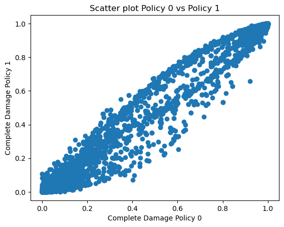
import matplotlib.pyplot as plt
# Scatter Plot
plt.scatter(bdmg_df_policies['DS_3_policy0'], bdmg_df_policies[f'DS_3_policy{i}'])
plt.title(f'Scatter plot Policy 0 vs Policy {i}')
plt.xlabel('Complete Damage Policy 0')
plt.ylabel(f'Complete Damage Policy {i}')
plt.savefig(f'CompleteDamage{i}.tif', dpi = 200)
plt.show()
Postprocessing: Recovery#
df_hhrs_policy2 = pd.read_csv (f"df_hhrs_results_policy_{i}.csv")
# merge household unit information with recovery results
pd_df_hs_policy2 = pd.merge(left = pd_df_policy2,
                    right = df_hhrs_policy2,
                    left_on=['guid','huid'],
                    right_on=['guid','huid'],
                    how='left')
pd_df_hs_policy2[['guid','huid']].describe()
| guid | huid | |
|---|---|---|
| count | 131987 | 131987 |
| unique | 104607 | 131987 |
| top | 6396008f-530a-481c-9757-93f7d58391f9 | B481677201001000H222 |
| freq | 293 | 1 |
6a) Sufficient Quality Solutions Found?#
pd_df_policy2 = pd.read_csv(f'pd_df_results_policy_{i}.csv')
df_hhrs_policy2 = pd.read_csv(f'df_hhrs_results_policy_{i}.csv')

pd_df_hs_policy2 = pd.merge(left = pd_df_policy2,
                    right = df_hhrs_policy2,
                    left_on=['guid','huid'],
                    right_on=['guid','huid'],
                    how='left')
# Add HHRS categories to dataframe
pd_df_hs_policy2 = add_label_cat_values_df(pd_df_hs_policy2,
            valuelabels = hhrs_valuelabels, variable = '13')
pd_df_hs_policy2 = add_label_cat_values_df(pd_df_hs_policy2,
            valuelabels = permanenthousing_valuelabels,
                        variable = '13')
poptable.pop_results_table(pd_df_hs_policy2,
                  who = "Total Population by Householder",
                  what = "by Permanent Housing at T=13 by Race Ethnicity",
                  where = "Galveston Island TX",
                  when = "2010 - Policy 2 - All buildings elvated",
                  row_index = 'Race Ethnicity',
                  col_index = 'Permanent Housing',
                  row_percent = '0 Not Permanent Housing'
                  )
| Permanent Housing | 0 Not Permanent Housing (%) | 1 Permanent Housing (%) | Total Population by Householder (%) | Percent Row 0 Not Permanent Housing |
|---|---|---|---|---|
| Race Ethnicity | ||||
| 1 White alone, Not Hispanic | 1,442 (58.7%) | 35,944 (60.8%) | 37,386 (60.7%) | 3.9% |
| 2 Black alone, Not Hispanic | 376 (15.3%) | 10,202 (17.3%) | 10,578 (17.2%) | 3.6% |
| 3 American Indian and Alaska Native alone, Not Hispanic | 14 (0.6%) | 242 (0.4%) | 256 (0.4%) | 5.5% |
| 4 Asian alone, Not Hispanic | 69 (2.8%) | 1,167 (2.0%) | 1,236 (2.0%) | 5.6% |
| 5 Other Race, Not Hispanic | 18 (0.7%) | 593 (1.0%) | 611 (1.0%) | 2.9% |
| 6 Any Race, Hispanic | 536 (21.8%) | 10,933 (18.5%) | 11,469 (18.6%) | 4.7% |
| 7 Group Quarters no Race Ethnicity Data | nan (nan%) | 48 (0.1%) | 48 (0.1%) | nan% |
| Total | 2,455 (100.0%) | 59,129 (100.0%) | 61,584 (100.0%) | 4.0% |
poptable.pop_results_table(pd_df_hs,
                  who = "Total Population by Householder",
                  what = "by Permanent Housing at T=13 by Race Ethnicity",
                  where = "Galveston Island TX",
                  when = "2010 - Baseline",
                  row_index = 'Race Ethnicity',
                  col_index = 'Permanent Housing',
                  row_percent = '0 Not Permanent Housing'
                  )
| Permanent Housing | 0 Not Permanent Housing (%) | 1 Permanent Housing (%) | Total Population by Householder (%) | Percent Row 0 Not Permanent Housing |
|---|---|---|---|---|
| Race Ethnicity | ||||
| 1 White alone, Not Hispanic | 1,046 (51.5%) | 8,572 (52.3%) | 9,618 (52.2%) | 10.9% |
| 2 Black alone, Not Hispanic | 376 (18.5%) | 2,799 (17.1%) | 3,175 (17.2%) | 11.8% |
| 3 American Indian and Alaska Native alone, Not Hispanic | 11 (0.5%) | 68 (0.4%) | 79 (0.4%) | 13.9% |
| 4 Asian alone, Not Hispanic | 63 (3.1%) | 566 (3.5%) | 629 (3.4%) | 10.0% |
| 5 Other Race, Not Hispanic | 14 (0.7%) | 202 (1.2%) | 216 (1.2%) | 6.5% |
| 6 Any Race, Hispanic | 521 (25.7%) | 4,153 (25.3%) | 4,674 (25.4%) | 11.1% |
| 7 Group Quarters no Race Ethnicity Data | nan (nan%) | 26 (0.2%) | 26 (0.1%) | nan% |
| Total | 2,031 (100.0%) | 16,386 (100.0%) | 18,417 (100.0%) | 11.0% |